Example Case Interview: the Kaggle Competition. (Part 2)
After finishing Part 1 of this tutorial we have our data features - recall that we saved the TF-IDF transformed text data from the names and description/caption fields and country names we got from the Geonames API in the ./data directory - we’ll assemble our training and test data matrices. After that, we’ll train an xgboost model comprised of trees and (briefly) tune a few hyperparameters.
It’s important to note that there are two different ways to train and validate a model: we can use the functions supplied to us in the xgboost package directly (e.g. xgb.train or xgb.cv), OR, we can use the caret package. I’ll illustrate both, but I’ll use caret to tune the model that will be used for making predictions on test.csv.
Go ahead and navigate to the run_classifier.R script to follow along!
(1) The assemble_data function
This function will load and format either your training or test data (from train.csv or test.csv accordingly). Namely, this data pre-processing function will do the following:
- Assembling training set: we change the good vector in
train.csvto zeros and ones for use with Xgboost’s function model training function,xgboost.train, append each of the the TF-IDF features from the name and description/caption text columns, append a one-hot encoding of the country names data, remove rows whose countries are missing (there are only about 150 of these cases), and return the training data and target vector with R’sas.matrixfunction. One-hot encoding of the country names will make one binary vector for each country name, and that vector will have a 1 if that row’s photo album came from the corresponding country. This is accomplished with the line
country_one_hot <- model.matrix(~ 0+country, data = country) - Assembling the test set: Again, we append text and one-hot encoded country features, only now we can ignore the target vector because we’re obviously missing good/bad photo albumn classifications. Also, instead of removing rows with missing country names, we’ll impute the most common country name (the USA) because we don’t have the luxury of just excluding albums from the test set. This imputation happens on the line
country$country[which(is.na(country))] <- names(which.max(table(country)))
Once you’re familiar with the assemble_data function, notice that the lines immediately after defining assemble_data are calling that function to gather our training set and training target vector:
train_data <- assemble_data()
train <- train_data$data; y <- train_data$y
(2.a) Train a model with randomly chosen parameters (optional)
If you want to use the model training, validation, and prediction functions supplied in the Xgboost package, that’s great, just be aware that you should supply each of xgb.train, xgb.cv, and xgb::predict with special data structures created with xgb.DMatrix instead of regular old matrices or R data.frames. First, we split up the train data into a training set and a validation set. I know, it’s confusing terminology - we’re taking 80% of the training data and calling this the training set and the remaining 20% the validation set. Anyway, the next chunk of code will fit a xgboosted tree model with a set of hyperparameters I pulled out of nowhere. Note that by using the watchlist setting, the training and validation set performance will print to the screen each time a new one of the nround small trees is appended to the aggregate model, but I’m saving this output to a text file via R’s sink function. Finally, we can estimate our accuracy on test.csv by using our prediction error on the validation set as a proxy:
trainIndex <- as.vector(caret::createDataPartition(y = y,
                                         p = 0.8, #fraction of training data kept as 'training' data
                                         list = FALSE))

#hyperparameters
max.depth <- 8 #How deep each weak learner (small tree) can get. Will control overfitting.
eta <- 0.5 #eta is the learning rate, which also has to do with regularization. 1 ->> no regularization. 0 < eta <= 1.
nround <- 150 #The number of passes over training data. This is the number of trees we're ensembling.

train.DMat <- xgb.DMatrix(data = train[trainIndex, ], label = y[trainIndex])

valid.DMat <- xgb.DMatrix(data = train[-trainIndex, ], label = y[-trainIndex])

#Fit boosted model with our random parameters. Save output that would otherwise print to console.
sink("./data/watchlist_output.txt", append = FALSE)
bst <- xgb.train(data = train.DMat,
                watchlist = list(train = train.DMat, validation = valid.DMat),
                max.depth = max.depth,
                eta = eta, nthread = 4,
                nround = nround,
                objective = "binary:logistic",
                eval_metric = "logloss")
sink()

valid.preds <- predict(bst, valid.DMat) #Xgboost::predict returns class probabilities, not class labels!
theta <- 0.5
valid.class_preds <- ifelse(valid.preds >= theta, 1, 0)
valid.accuracy <- sum(as.numeric(valid.class_preds == y[-trainIndex]))/length(y[-trainIndex]) #~78% valid accuracy
print(sprintf("Accuracy on validation set: %f", valid.accuracy))
Before moving on, one cool feature of boosted tree models is that we can get variable importances - a variable’s importance to the overall model is an average of the improvement in accuracy gained from all of the small trees every time that feature was used to split up a node in a tree. Viewing the variable importances might help to verify that your model makes sense, and it wouldn’t hurt to include it in a code/case interview to demonstrate that you can put words behind the model you’ve built.
importance_matrix <- xgb.importance(model = bst, feature_names = colnames(train))
print(importance_matrix)
barplot(importance_matrix$Gain[6:1],
        horiz = T,
        names.arg = importance_matrix$Feature[6:1],
        main = "Estimated top 6 features by accuracy gain",
        cex.names = .6)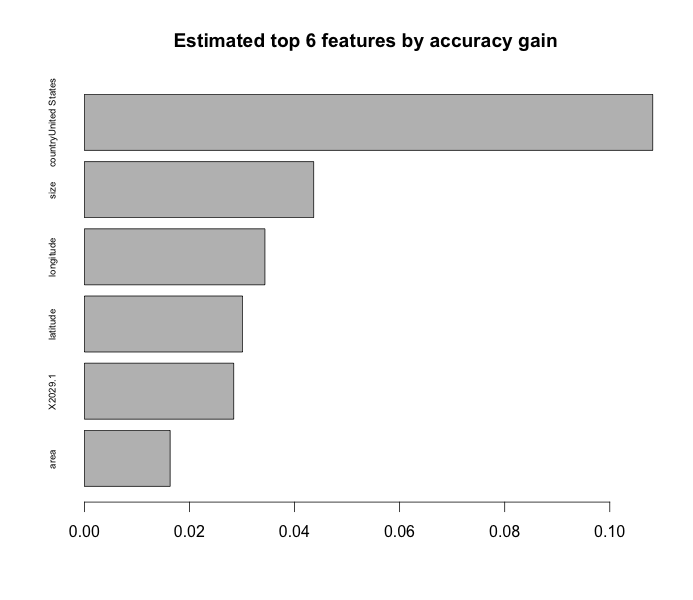
(2.b) Tune hyperparameters with caret::train
Since we really have little insight into whether we should use a small max_depth or a large one, let all of our features be available when constructing a weak learner (i.e. how to set colsample_bytree), etc… We should set up a grid of parameters, cross validate a model for every combination of parameters in the grid, and pick the best one! This is a very computationally expensive way to pick a model, and note that it’s still not even very refined when there are big discrete gaps in the hyperparameter values present in the grid. Still, we might be able to eek out better performance with a high-level gridsearch. Use R’s convenient expand.grid function to make a data.frame with every combination of hyperparameters you’re interested in; use caret::trainControl to specify the type of validation you’re interested in (we’ll do 5-fold cross validation); and use caret::train to search over the grid of hyperparameter combinations to find the model that minimizes log-loss. We can only use caret because it recently began supporting model = 'xgbTree' (caret supports hundreds of different models, actually), and it conveniently supports log-loss as an optimization metric too!
xgb_grid <- expand.grid(nrounds = c(100),
                        eta = c(0.2),
                        max_depth = c(7, 10),
                        colsample_bytree = c(0.6, 1),
                        gamma = c(0.75, 1),
                        min_child_weight = c(1))

tr_control <- caret::trainControl(method = "cv",
                          number = 5,
                          classProbs = TRUE,
                          allowParallel = TRUE,
                          summaryFunction = mnLogLoss, #Using summaryFunction = summaryFunction will use ROC (i.e. AUC) to select optimal model. We want log-loss.
                          verboseIter = TRUE)

xgb_cv1 <- caret::train(x = train,
                       y = as.factor(ifelse(y==1, "good", "bad")), # Target vector should be non-numeric factors to identify our task as classification, not regression.
                       tuneGrid = xgb_grid, #Which hyperparameters we'll test.
                       trControl = tr_control, # Specify how cross validation should go down.
                       method = "xgbTree",
                       metric = "logLoss", # Convenient.
                       maximize = FALSE) # We want to minimize loss, after all.
A couple of points regarding caret’s functionality versus xgboost’s: first, you’ll need to make y a factor vector instead of a numeric vector so that caret::train knows that you want to perform a classification task instead of a regression task. Also, with caret we can return to using matrices and data.frames instead of xgb.DMatrix’s. Finally - this gridsearch will take a long time (at least 3 hours on a Macbook with an i7 core processor).
(3) Visualize performance with an ROC curve (optional):
Receiver operating characteristics (ROC’s) are confusing, so I suggest reading the Wikipedia article about them. Maybe I’ll make a post about it soon. Basically, they just let you compare the performance of different classification models. A popular one called “area under curve” the false positive rate (i.e. rate at which we call a bad photo album good) versus the true positive rate (i.e. rate at which we call good albums good). When the false positive rate (FPR) is zero, we’ve just called every album ‘bad’ so the true positive rate (TPR) is 0%. Similarly, when we call every album good, the FPR is 100% and the TPR 100%. The best model ever would have 0% FPR and 100% TPR, so an “area under the curve” of 1. I suggest reading this great intro link about AUC and ROC curves. Anyway, you need to obtain class probabilities from caret::train or xgb.predict in order to build an ROC curve.
My code in run_classifier.R will let you build the ROC curve by hand as well as leverage the R packages pROC and ROCR for simplification:
auc_est <- pROC::auc(y[-trainIndex], valid.preds$good) #0.8638 on the validation set, not bad...

rocr_pred <- prediction(valid.preds$good, y[-trainIndex])
rocr_perf <- performance(rocr_pred, measure = "tpr", x.measure = "fpr") #this is of class "performance," it's not a list
auc_data <- data.frame("fpr" = unlist(rocr_perf@x.values), "tpr" = unlist(rocr_perf@y.values))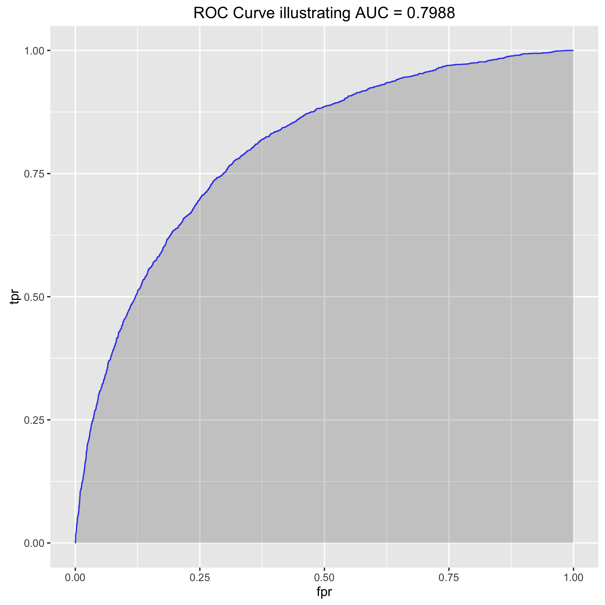
(4) Assemble test data and gather predictions
Just like in step (1), use assemble_data to construct the test set with all of the new features we have. If you look in the example_entry.csv file that the Kaggle administrator supplied, they want for the output to have two columns, id and good, where good is binary 0/1. Since caret::predict(model, newdata, type = "raw") returns factor variables representing class membership, just use R’s super-convenient ifelse function to change the results to zeros and ones. Save the data, and submit!
test_data <- assemble_data(train_or_test = "test",
                          data_file = "./data/test.csv",
                          name_tfidf_file = "./data/test_name_tfidf.rds",
                          desc_caption_tfidf_file = "./data/test_desc_caption_tfidf.rds",
                          country_file = "./data/aggregate_test_countries.RDS")

test <- test_data$data
test_classes <- ifelse(predict(xgb_cv1, test, type = "raw") == "good", 1, 0)

#Save and then submit predictions!
write.csv(data.frame(id = read.csv("./data/test.csv")$id, good = test_classes),
          "./output/test_predictions.csv", row.names = FALSE)
(Optional) run this bad boy yourself
From your command line, navigate to the photo_kaggle directory and run > Rscript ./scripts/run_classifier.R. This will build an xgboost model and save predictions from the test.csv file provided to us on Kaggle. From here it’s easy to add and tune more hyperparameters, add some creative features, delete useless ones, etc. Xgboost is really powerful, have fun!