The inner workings of the lambdarank objective in LightGBM
The ranking objective
The ability to sort-order items in a list in an optimal way, often referred to as learning to rank (or LETOR), is sort of the forgotten middle child supervised machine learning. It’s not directly regression, but some LETOR solutions can involve regression. It’s not exactly binary classification, but several popular LETOR models are closely related to binary classification. Some LETOR models involve assigning probabilities to ranking permutations. And then the metrics for evaluating “well-ranked” like NDCG and ERR are much more involved than the standard precision, recall, or RMSE just don’t cut it.
When I first got involved with LETOR models, I found a lot of the literature to be kind of chaotic. Specifically, the foundational writings on LETOR by Burges[4] I found very difficult to follow just from a notational standpoint. I knew that LightGBM supported the lambdarank objective, but it took time to fully grasp the connection between papers about pairwise loss, lambdarank gradients, and LightGBM’s actual LambdaMART implementation in C++. So in this post I’ll try to cover the core principals of what the lambdarank objective is, and then I’ll dive into exactly what’s going on in the LambdarankNDCG optimization function used by LightGBM to estimate LamdbaMART models.
Eventually we’ll be getting into the LightGBM C++ source code available on GitHub here.
Why learning to rank is hard
The number one reason why LETOR is harder than the more traditional supervised learning tasks is that the data is hierarchical. In continuous regression or binary/multiclass/multilabel classification, we map one input vector to one output vector. Each input is typically assumed to be distributed $IID$. When we rank items within a list, our units of measure (items) are not independent of each other, but instead are differentially ranked relative to each other. It’s not even that the ranking models needs to output probabilities or estimates of some conditional mean $E[Y|X]$ - it only needs to output values that allow us to sort items within a list in an optimal order. A model that outputs the scores ${-\infty, 0, \infty}$ for three items (respectively) would provide the exact same ranking as a model that outputs scores ${-0.01, -0.005, -0.001}$ for each of those same products.
LETOR training data is often stored in the SVMlight format, which comes from T. Joachim’s SVMRank model and corresponding ML software written in C [1]. The SVMLight format basically reserves the first column for the dependent variable, the second column for what it calls the qid, or the group identifier, and then all other columns are reserved for feature values. So LETOR shares a similar data structure really to how we would need to shape data as input into RNN/LSTM models: (samples, time steps, $y$). One sample is comprised of multiple products within a single query, like this:
| Y | qid | feature_0 | feature_1 | feature_2 | feature_3 |
|---|---|---|---|---|---|
| 0 | 0 | 12.2 | -0.9 | 0.23 | 103.0 |
| 1 | 0 | 13.0 | 1.29 | 0.98 | 93.5 |
| 2 | 0 | 14.0 | 1.29 | 0.98 | 93.5 |
| 0 | 0 | 11.9 | 1 | 0.94 | 90.2 |
| 1 | 1 | 10.0 | 0.44 | 0.99 | 140.51 |
| 0 | 1 | 10.1 | 0.44 | 0.98 | 160.88 |
Pairwise loss starts with binary classification
The lambdarank LightGBM objective is at its core just a manipulation of the standard binary classification objective, so I’m going to begin with a quick refresher on classification here.
Start by considering two items within a query result set, call them items $i$ and $j$. Assume that $Y_{i} > Y_{j}$, i.e. that item $i$ is more relevant than item $j$. Suppose that these items can also be represented by feature vectors $X_{i}$ and $X_{j}$, respectively. A model, referred to as $f(\cdot)$, minimizes pairwise classification loss by minimizing the number of pairwise inconsistencies. When $Y_{i} > Y_{j}$, a good model will provide us output values $s_{i}, s_{j}$ such that $s_{i} = f(X_{i}) > f(X_{j}) = s_{j}$.
Then logically, pairwise loss should be large when $s_{i} - s_{j} < 0$ and small when $s_{i} - s_{j} > 0$. We can use this difference to model the probability in a binary classification model that the pair $(i, j)$ as “$Y=1$” or $(j, i)$ as “$Y=0$”. This classification model will maximize the Bernoulli likelihood, $\mathcal{L}$, given the data consisting of all pairs $(i, j)$ where $Y_{i} > Y_{j}$. The Bernoulli likelihood parameterized by $\theta = Pr(y|x)$, is expressed as
\begin{align} \mathcal{L} = \theta^{y}(1 -\theta)^{1-y}, \hspace{5mm} y \in {0, 1} \end{align}
Since $\log(\cdot)$ is a monotone transformation - a fancy way of saing that $5 < 6 \rightarrow \log(5) < \log(6)$ - then maximizing Bernoulli likelihood and log-likelihood is the same thing. Log-likelihood, or $\ell\ell$ is given by
\begin{align} \ell\ell = \log(\mathcal{L}) = y\log(\theta) + (1-y)\log(1 - \theta) \end{align}
We typically express $Pr(y_{ij}|s_{i}, s_{j})$ via the logistic function: $Pr(y_{ij}|s_{i}, s_{j}) = \frac{1}{1 + e^{-\sigma(s_{i} - s_{j})}}$ because it’s easy to differentiate and it gives us a way to smush pairwise model scores $s_{i}-s_{j}$ from $(-\infty, \infty)$ to the probability scale [0, 1]. The constant $\sigma$ it typical to set $\sigma=1$, but LightGBM exposes this as a hyperparameter named sigmoid, so I’ll keep it in the notation.
\begin{align} \ell\ell_{ij} &= y_{ij}\log(\frac{1}{1 + e^{-\sigma (s_{i} - s_{j})}}) + (1 - y_{ij})\log(\frac{e^{-\sigma(s_{i} - s_{j})}}{1 + e^{-\sigma(s_{i} - s_{j})}}) \end{align} \begin{align} &= -y_{ij}\log(1 + e^{-\sigma (s_{i} - s_{j})}) + \log(e^{-\sigma (s_{i} - s_{j})}) - \log(1 + e^{-\sigma (s_{i} - s_{j})}) - y_{ij}\log(e^{-\sigma (s_{i} - s_{j})}) + y_{ij}\log(1 + e^{-\sigma (s_{i} - s_{j})}) \end{align} \begin{align} &= (1 - y_{ij})\log(e^{-\sigma (s_{i} - s_{j})}) - y_{ij}\log(1 + e^{-\sigma (s_{i} - s_{j})}) \end{align}
If maximizing $\ell \ell_{ij}$ is good, then minimizing $-\ell \ell_{ij}$ must also be good. Machine learning practicioners commonly refer to -1 times the loglikelihood as logloss:
\begin{align} \text{logloss}_{ij} = (y_{ij}-1)\log(e^{-\sigma (s_{i} - s_{j})}) + y_{ij}\log(1 + e^{-\sigma (s_{i} - s_{j})}) \end{align}
In the literature on pairwise loss for ranking, right here is where I’ve witnessed a slight of hand: we only need to learn from the cases where $y_{ij} = 1$. This is because negative cases are symmetric; when $Y_{i} > Y_{j}$ (meaning that the pair $(i, j)$ has the label $y=1$), this implies that $(j, i)$ has label $y=0$. Training on tied pairs doesn’t help, because the model is trying to discern between relevant and irrelevant items. Therefore, all we really need to keep are the instances of $y_{ij}=1$, and the pairwise logloss expression can be simplified.
\begin{align} \text{logloss}_{ij} = \log(1 + e^{-\sigma (s_{i} - s_{j})}) \end{align}
This loss is also known as “pairwise logistic loss,” “pairwise loss,” and “RankNet loss” (after the siamese neural network used for pairwise ranking first proposed in [2]).
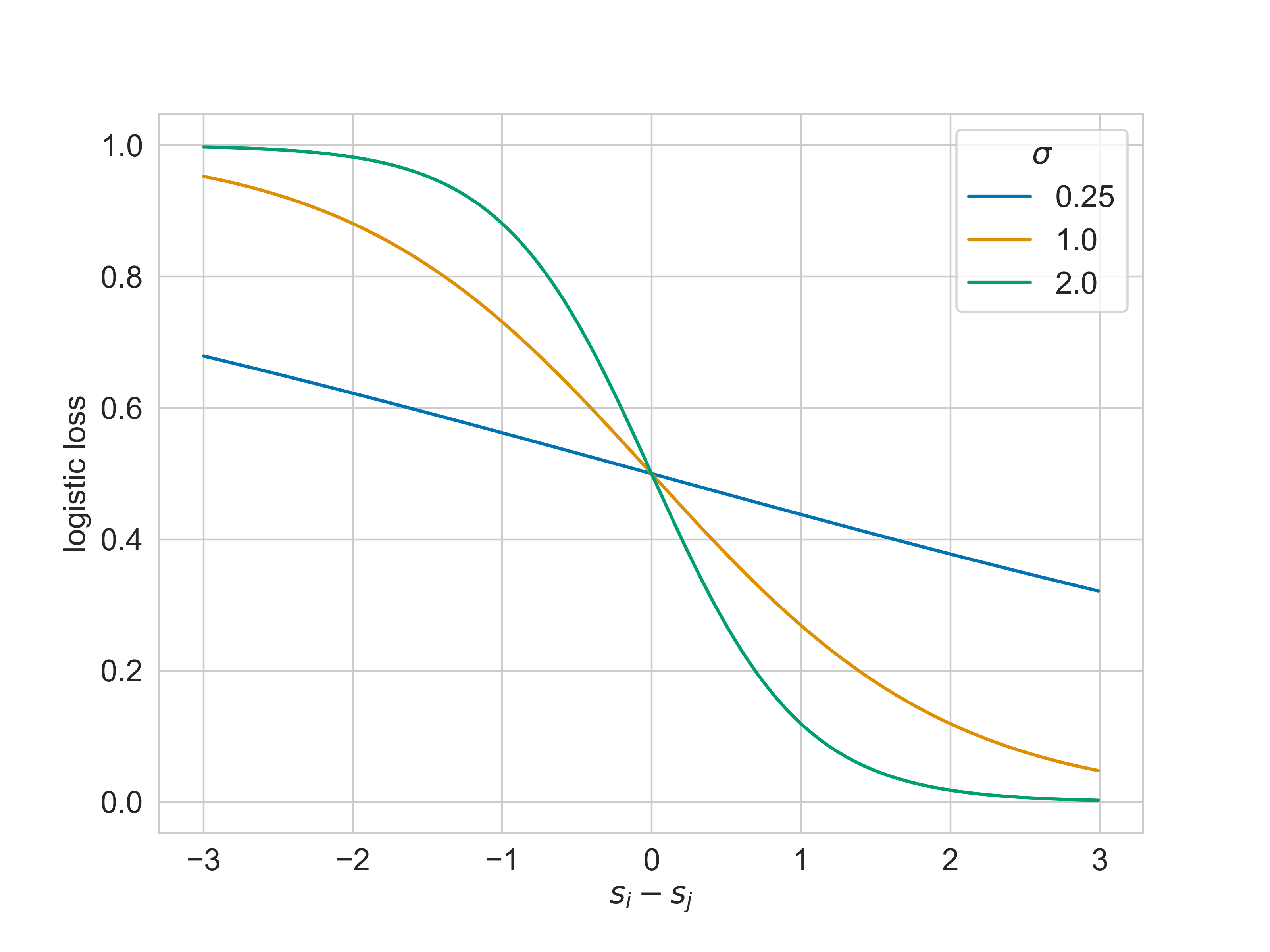
It’s not too difficult to understand: when $Y_{i} > Y_{j}$, the model will achieve small loss when it can predict scores $s_{i} - s_{j} > 0$. The loss will be large when $s_{j} > s_{i}$. The gradient of the loss for any $s_{i} - s_{j}$ is also controlled by $\sigma$. Larger values of $\sigma$ penalize pairwise inconsistencies than values closer to zero.
LightGBM implements gradient boosting with the lambdarank gradient
LightGBM is a machine learning library for gradient boosting. The core idea behind gradient boosting is that if you can take the first and second derivatives of a loss function you’re seeking to minimize (or an objective function you’re seeking to maximize), then LightGBM can find a solution for you using gradient boosted decision trees (GBDTs). Gradient boosting is more or less a functional version of Newton’s method, which is why we need the gradient and hessian. During training it builds a sequence of decision trees each fit to the gradient of the loss function when the model is evaluated on the data at the current boosting iteration.
\begin{align} \frac{\partial \text{logloss}_{ij}}{\partial s_{i}} &= \frac{-\sigma e^{-\sigma(s_{j} - s_{i})}}{1 + e^{-\sigma(s_{i} - s_{j})}} \end{align} \begin{align} &= \frac{-\sigma}{1 + e^{\sigma(s_{i} - s_{j})}} \hspace{10mm} (\text{mult by} \hspace{1mm} \frac{e^{\sigma(s_{i} - s_{j})}}{e^{\sigma(s_{i} - s_{j})}}) \end{align} \begin{align} &= \lambda_{ij} \end{align}
This is where the “lambda” in lambdarank comes from.
Note a critical shortcoming of the $\lambda_{ij}$ gradients - they are completely positionally unaware. The formulation of the pairwise loss that we’ve used to derive the $\lambda_{ij}$ treats the loss the same whether we’ve incorrectly sorted two items near the top of the query or near the bottom of the query. For example, it would assign the same loss and gradient to the pairs $(1, 3)$ and $(100, 101)$ when $s_{i} - s_{j}$ and $Y_{i}$ and $Y_{j}$ are the same. But most eCommerce or Google/Bing users spend like 90% of their time near the top of the query, so it’s much more important to optimze the items appearing within the first few positions. A possible correction proposed by Burges in 2006 [4] was to just scale $\lambda_{ij}$ by the change in NDCG (a positionally-aware ranking metric) that would be incurred if the incorrect pairwise sorting of items $(i, j)$ was used:
\begin{align} \lambda_{ij} = \log(1 + e^{-\sigma (s_{i} - s_{j})})|\Delta NDCG_{ij}| \end{align}
This is known as the lambdarank gradient. The claim is that by using this form of the gradient within a loss minimization procedure, we end up maximizing NDCG. Well, if this decision to scale the original $\lambda_{ij}$ by $|\Delta NDCG_{ij}|$ seems kind of arbitrary to you, you are not alone. Several researchers have taken issue with it, viewing it more as a hack than a true gradient of a real loss function [7]. Just know that the term lambdarank does not refer to a loss function (like some other LightGBM objective strings like "mse" or "mape"), but to an explicit gradient formulation.
Anyway, we have the positionally-aware “gradient” of the pairwise loss function with respect to a single product-product pair $(i, j)$ of differentially-labeled products. LightGBM and GBDTs generally regress decision trees on the loss gradients computed with respect to individual samples (or rows of a dataset), not single products within pairs of products.
In order to just get the gradient with respect to product i, we have to accumulate the gradient across all pairs of products where $i$ is the more-relevant item, and symmetrically, across all pairs where $i$ is the less-relevant item. Let $I$ refer to the set of item pairs $(i, j)$ where the first item is more relevant than the second item.
\begin{align} \lambda_{i} = \sum_{j:{i, j} \in I}\lambda_{ij} - \sum_{j:{j, i} \in I}\lambda_{ij} \end{align}
We need to take a quick detour. Confusingly, LightGBM (as well as XGBoost) are known as gradient boosted tree learning libraries. They actually implement Newton boosting [3]. Gradient boosting is premised on taking a first-order Taylor approximation of the loss function about the current estimates of the loss at each step of the tree-estimation process. But you can get better results by taking higher-order approximations to the loss function, and LightGBM uses a second-order approximation. In basic gradient boosting, during each boosting iteration we fit a new decision tree directly to $Y = g_{i}^{k}$, where $g_{i}^{k} = \lambda_{i}^{k}$, the gradient of the loss of the model on iteration $k$. But in Newton boosting, the regression involves both the hessian (designated $h_{i}^{k}$) and the gradient:
\begin{align} \text{tree}_{k+1} = \arg\min\sum_{i=1}^{n}h_{i}^{k}\big(-\frac{g_{i}^{k}}{h_{i}^{k}} - \ell\ell_{i}^{k}\big)^{2} \end{align}
Since we’ve only derived the first derivative of the loss, let’s find the second derivative by applying the quotient rule:
\begin{align} \frac{\partial^{2} \text{logloss}_{ij}}{\partial s_{i}^{2}} &= \frac{\sigma^{2}e^{-\sigma(s_{j} - s_{i})}|\Delta NDCG_{ij}|}{(1 + e^{-\sigma(s_{j} - s_{i})})^{2}} \end{align} \begin{align} &= \frac{-\sigma}{1 + e^{-\sigma(s_{j} - s_{i})}}|\Delta NDCG_{ij}| \cdot \frac{-\sigma e^{-\sigma(s_{j} - s_{i})}}{1 + e^{-\sigma(s_{j} - s_{i})}} \end{align} \begin{align} &= \lambda_{ij}\frac{-\sigma e^{-\sigma(s_{j} - s_{i})}}{1 + e^{-\sigma(s_{j} - s_{i})}} \end{align}
And we’re done with the math! Later on we’ll map these components of the gradient and hessian to the actual C++ code used in LightGBM’s actual lambdarank objective source code.
Pointwise, pairwise, or listwise?
A very confusing aspect of the lambdarank gradient is that despite being closely related to the gradient of the classic pairwise loss function, a LightGBM LGBMRanker model can score individual items within a query. It does not expect for two inputs to be provided as ranking input like rnk.predict(x1, x2). Further, the calculations required to derive the gradient, $\frac{\partial \text{logloss}}{\partial s_{i}}$ involves sums over all pairs of items within a query, as if it were a listwise LETOR algorithm.
The fact is that the lambdarank LightGBM gradient is based on pairwise classification, but a lambdaMART model involves fitting decision trees to gradients computed g all pairs of differentially-labeled items within a query. Each individual item (each row in the training data) is assigned its own gradient value, and then LightGBM simply regresses trees on those gradients. This is why we can score individual items like rnk.predict(x1):
import lightgbm as lgb
import numpy as np

np.random.seed(123)
X = np.random.normal(size=(100,5))
y = np.random.choice(range(4), size=100, replace=True)
grp = [10] * 10

rnk = lgb.LGBMRanker(objective='lambdarank')  # lambdarank is actually default objective for LGBMRanker
rnk.fit(X, y, group=grp)

rnk.predict(X[50, :].reshape(1, -1))  # pointwise score for row 50
array([-1.95225947])
Other researchers have tried to develop better intuitions and better categorizations of LETOR models other than pointwise/pairwise/listwise. The best exploration of this topic I’ve found is Google’s 2019 paper on Groupwise Scoring Functions [5] which provides the foundation for the popular Tensorflow Ranking library. The paper provides the notion of a scoring function, which is different than the objective/loss function. A LambdaMART model is a pointwise scoring function, meaning that our LightGBM ranker “takes a single document at a time as its input, and produces a score for every document separately.”
How objective functions work in LightGBM
You might be used to interacting with LightGBM in R or Python, but it’s actually a C++ library that just happens to have well built-out R and Python APIs. Navigate to src/objectives and you’ll see the implementations of specific objective/loss functions such as rank_objective.cpp in addition to objective_function.cpp which implements a objective class factory.
Each individual objective class must define a method named GetGradients that can update model score (aka “loss”) values, gradients, and hessians. Each objective file may contain multiple objective classes. The GDBT class contained within boosting/gbdt.cpp that actually calls GetGradients to fit regression trees within LightGBM’s main training routine.
In rank_objective.cpp, GetGradients just iterates over queries in the training set, calling an inner GetGradientsForOneQuery that calculates the pairwise loss and lambdarank gradients/hessians for each item within each query.
void GetGradients(const double* score, score_t* gradients,
                    score_t* hessians) const override {
    for (data_size_t i = 0; i < num_queries_; ++i) {
        const data_size_t start = query_boundaries_[i];
        const data_size_t cnt = query_boundaries_[i + 1] - query_boundaries_[i];
        GetGradientsForOneQuery(i, cnt, label_ + start, score + start,
                                gradients + start, hessians + start);
        ...
    }
}

virtual void GetGradientsForOneQuery(data_size_t query_id, data_size_t cnt,
                                     const label_t* label,
                                     const double* score, score_t* lambdas,
                                     score_t* hessians) const override {
    // score, lambdas, and hessians are modified in-place...
}
There are actually a couple of different ranking objectives offered by LightGBM that each subclass a RankingObjective wrapper class:
LambdarankNDCG: this is the selected objective class when you setLGBMRanker(objective="lambdarank").RankXENDCG: Rank-cross-entropy-NDCG loss ($XE_{NDCG}$ for short) is a new attempt to revise the lambdarank gradients through a more theoretically sound argument that involves transforming the model scores $s_{i}$ into probabilities and deriving a special form of multiclass log loss [6].
Connecting the math to the code
All of the lambdarank math is located primarily in two methods within the LambdarankNDCG objective class:
GetSigmoidperforms a look-up operation on a pre-computed, discretized logistic function: \begin{align} \frac{\lambda_{ij}}{|\Delta NDCG_{ij}|} &= \frac{1}{1 + e^{\sigma(s_{i} - s_{j})}} \end{align} stored in a vector namedsigmoid_table_. Using pre-computed logistic function values reduces the number of floating point operations needed to calculate the gradient and hessian for each row of the dataset during each boosting iteration.GetGradientsForOneQuerypasses $(s_{i} - s_{j})$ toGetSigmoid, which applies a scaling factor to transform $(s_{i} - s_{j})$ into an integer value (of typesize_tin C++) so that can then be used to look up the corresponding value withinsigmoid_table_.GetGradientsForOneQueryprocesses individual queries. This method launches twoforloops, the outer loop iterating fromi=0totruncation_level_(a reference to thelambdarank_truncation_levelparameter) and the inner loop iterating fromj=i+1tocnt, the latter being the number of items within the query at hand. This is where the math comes in:
// calculate lambda for this pair
double p_lambda = GetSigmoid(delta_score);              // 1 / (1 + e^(sigma * (s_i - s_j)))
double p_hessian = p_lambda * (1.0f - p_lambda);        // Begin hessian calculation.
// update
p_lambda *= -sigmoid_ * delta_pair_NDCG;                // Finish lambdarank gradient: -sigma * |NDCG| / (1 + e^(sigma * (s_i - s_j)))
p_hessian *= sigmoid_ * sigmoid_ * delta_pair_NDCG;     // Finish hessian calculation. See derivation below.
Let’s tie the code together with the math, as I had particularly struggled to understand why p_hessian = p_lambda * (1 - p_lambda) was valid:
\begin{align} \text{p_lambda} &= \frac{1}{1 + e^{\sigma(s_{i} - s_{j})}} \end{align} \begin{align} 1 - \text{p_lambda} &= \frac{e^{\sigma(s_{i} - s_{j})}}{1 + e^{\sigma(s_{i} - s_{j})}} \end{align} \begin{align} \text{p_lambda}(1 - \text{p_lambda}) &= \frac{e^{\sigma(s_{i} - s_{j})}}{(1 + e^{\sigma(s_{i} - s_{j})})^{2}} \end{align} \begin{align} \Rightarrow \frac{\partial^{2}\text{logloss}}{\partial s_{i}^{2}} &= \sigma^{2}|\Delta NDCG_{ij}|\text{p_lambda}(1 - \text{p_lambda}) \end{align}
And that’s just about it! There are some other tweaks that some LightGBM contributors have made, such as the option to “normalize” the gradients across different queries (controlled with the lambdarank_norm parameter), which helps prevent the case where one very long query with tons of irrelevant items gets an unfair “build-up” of gradient value relative to a shorter query.
References
[2] Burges, et al., 2005. Learing to Rank using Gradient Descent
[3] Sigrist, 2020. Gradient and Newton Boosting for Classification and Regression
[4] Burges, 2010. From RankNet to LambdaRank to LambdaMART: An Overview
[5] Ai, Wang, Bendersky et al., 2019. Learning Groupwise Scoring Functions Using Deep Neural Networks
[6] Bruch, 2021. An Alternative Cross Entropy Loss for Learning-to-Rank
[7] Wang, Li, et al., 2018. The LambdaLoss Framework for Ranking Metric Optimization