Introduction

Oftentimes us data scientists find ourselves presented with a new, foreign dataset (or set of files that jointly comprise a new dataset), with the goal simply to “build a model.” Model interpretability in a case like may fall to the wayside, and this is especially true when the data have been anonymized and we’re really not supposed to understand the meaning of any particular data point or field name.

In a high-dimensional setting (hundreds, thousands of potential features to choose from) with little understanding the individual fields, we face three main challenges when it comes to building a model:

1. Diverse data processing needs: numeric and categorical features require different data processing steps, as do features with a lot of missing data
2. Feature selection: sifting signal through the noise without making arbitrary and capricious decisions when it comes to selecting features into a resulting model
3. Building a reusable data and modeling pipeline: Getting predictions from a new dataset should not require having to call dozens of custom functions in the correct order in order to transform the data into the format expected by the model. This process needs to be as easy as calling a single .transform method.

This post is about how I built one Sklearn Pipeline that can take me from read_csv resulting in hundreds of anonymous features to a completely processed data ready for model predictions with the call of single method.

The data, the code

You’ll need to download the IEEE-CIS Fraud Detection data from Kaggle. All of the code required to follow along is in my GitHub repo: ieee-cis-fraud-detection

Files you’ll need: train_transaction.csv test_transaction.csv

Note that I’m ignoring the *_identity.csv files. We can get pretty decent performance (90% precision, 50% recall) from the transactions data alone.

Pipelines and Transformers: DataFrame to model matrix in one go

Sklearn Pipelines are structures that allow Data Scientists to concatenate different data transformation tasks (called “steps”) out of Transformer objects. A Pipeline can end in Sklearn Estimator that fits a model.

For example, we can define a simple Pipeline that imputes missing values with the median, scales all $X$ variables between 0 and 1, and then fits a Random Forest:

from sklearn.pipeline import Pipeline
from sklearn.impute import SimpleImputer
from sklearn.preprocessing import MinMaxScaler
from sklearn.ensemble import RandomForestClassifier
from pandas import read_csv

step1 = ('impute', SimpleImputer(strategy='median')
step2 = ('01scaler', MinMaxScaler())
step3 = ('rf', RandomForestClassifier(n_estimators=10))
pipeline = Pipeline(steps = [step1, step2, step3])

X = read_csv('path/to/training/data.csv')
pipeline.fit_transform(X)

The real trick to getting started with Pipelines is that all but the final step must have both a .fit and a .transform method (e.g. the MinMaxScaler transformer), but the last step just needs a .fit method. This lets the final step be a an Estimator (a model), instead of a data Transformer.

At the end of the day, I really wanted to know just how far can I go with Sklearn Pipelines? Can I do all of my data processing tasks within a single transformer Pipeline? Given a new batch of data, I didn’t want to have to recreate the full training data creation process - running a bunch of one-off Data Scientist-defined data processing functions in a very specific order. My goal: could I go from pandas.read_csv to model predictions in a single line of code?

Feature engineering: diverse needs

I ended up building the following data processing Pipeline

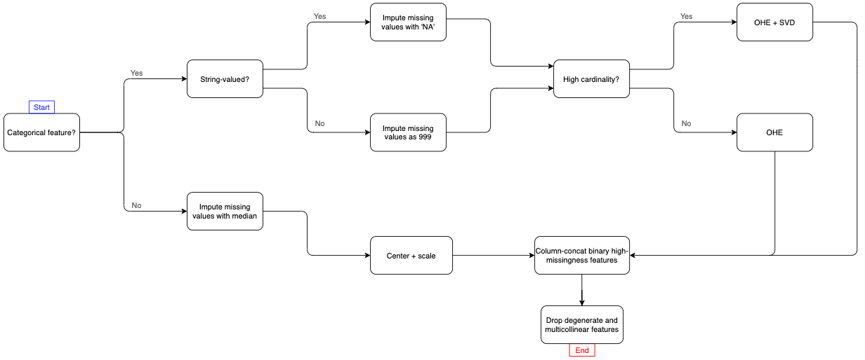
This is end-to-end – there are only two steps:

1. Load a IEEE-CIS Fraud dataset into a pandas.DataFrame
2. Pass that data to the pipeline and execute .fit_transform. The Pipeline will handle every data processing and feature engineering step.

The main complexities in building a one-stop-shop like this is that we have a diversity of needs because of all of the different types of features present in the IEEE-CIS dataset. Namely, categorical features generally pose a few issues, and as you can see in the Pipeline flowchart above, I had to break up the IEEE data into 5 groups:

1. Continuous (“numeric”) features. These features will be processed in their own Pipeline.
2. Categorical features will be processed in their own Pipeline.
   • 2.1 String-valued categorical features with low cardinality, e.g. the credit card someone used in a transaction like “mastercard” or “visa”, with fewer than 20 unique categorical levels.
   • 2.2. String-valued, high-cardinality features.
   • 2.3. Numerically-valued, low-cardinality features, e.g. a feature whose levels are numbers that represent categories.
   • 2.4. Numerically-valued, high-cardinality features.

Imputing missing values: we’ll impute missing values in string-valued categorical features with the string ‘NA’ and in numerically-valued categorical features with the number 999. We impute numeric features with their respective medians.

One-hot encoding: once both string and numerically-valued features have had their missing values imputed, next, we consider features with fewer than 20 unique levels as “low cardinality”. These features will simply be one-hot encode these into binary indicator columns.

For “high cardinality” features we’ll one-hot encode them into a very wide, very sparse binary matrix, and then use the SVD to embed that sparse matrix into a smaller dense matrix. We do this as opposed to constructing potentially thousands or tens of thousands of binary features. This is basically a method of categorical feature embedding.

The categorical and continuous pipelines will be concatenated “additively” or “horizontally” using the sklearn.pipeline.FeatureUnion pipeline composition function. Finally, we add some processing on top of the union of the categorical and continuous pipelines to drop redundant (read: highly correlated) features and features with very little variance, like this:

# -- continuous feature pipeline
num_pipeline = numeric_feature_pipeline(df
                                        , numeric_features=num_features)

# -- categorical feature pipeline
cat_pipeline = categorical_feature_pipeline(df
                                            , categorical_string_features=cat_str_features
                                            , categorical_numeric_features=cat_num_features
                                            , high_cardinality_cutoff=data_config.hi_cardinality_cutoff)
# -- the full feature pipeline
feature_pipeline = Pipeline(steps=[('preprocess', FeatureUnion([('categorical', cat_pipeline)
                                                                , ('numeric', num_pipeline)]))
                                    , ('decorrelate', UncorrelatedFeatureSelector())
                                    , ('nondegenerate', NonDegenerateFeatureSelector())])

# -- fit feature pipeline, transform training data
X_train = feature_pipeline.fit_transform(read_csv('path/to/training/data.csv'))                  

While not encountered in this dataset, ordinal categorical features (features whose levels imply a specific ranking, e.g. “cold” < “warm” < “hot”) require additional special attention.

Step 2: processed features into a model

Most examples of Sklearn Pipelines’ final step is an Sklearn Estimator, so that feature engineering steps feed directly into a predictive model. While this makes sense for simple, quick-to-fit Pipelines, the Pipeline I’ve laid out above takes about 8 minutes to fit and transform my training set of ~500,000 training examples. Therefore, we’ll feature_pipeline unto itself, apart from a subsequent model.

Benchmark classifier

It’s generally accepted that Data Scientists should try to avoid needless model complexity if it is precisely that, needless. If a simple, easily-interpreted benchmark model can perform just as well as a more complex, tree- or neural-network-based model, then stick with the benchmark model.

The LASSO model is a first stop on your way to building the right predictive model. The LASSO linear model is a penalized regression model that has the benefit of sparsity (it selects only important features from a set of superfluous features) and interpretability (this is a linear model with traditional linear coefficients), and it comes in flavors that support both classification and continuous regression tasks.

As is the case with most types of predictive models, the LASSO model comes with a set hyperparameters, the most important of which is C, the inverse of the L1-penalty weight. Smaller values of C result in more sparsity (fewer features selected), and C = infinity is equivalent to a regular old logistic regression. Best practices are to use a search procedure in tandem with cross-validation to pick out the value of C that will allow our model to generalize the best to unseen test-set data. For that, we use Sklearn’s sklearn.model_selection.GridSearchCV cross-validation procedure.

The coolest thing about GridSearchCV is that it provides the ability to automatically refit a model on all of the training data using the best parameter setting found at the conclusion of the hyperparameter search.

# -- define classifier object and hyperparameter grid
model = LogisticRegression(penalty='l1'
                           , solver='liblinear'
                           , class_weight='balanced')
param_grid = {'C'=[0.1, 1, 10]}

# -- search grid using cross-validation, refit on all training data 
gcv = GridSearchCV(model
                   , param_grid=param_grid
                   , cv=3
                   , n_jobs=2
                   , scoring=['f1', 'roc_auc', 'recall', 'precision', 'accuracy']
                   , refit='f1'
                   , verbose=10)
gcv.fit(X_train
        , y=y_train)

# -- fitted model on best parameter set
best_model = gcv.best_estimator_

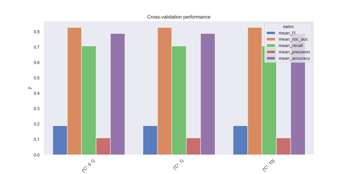
As we can see, our hyperparameter search does not accomplish much - cross-validated model performance is constant over our three choices of C. We can generally expect low precision, about 0.1, meaning that most of the LASSO model’s fraud alerts will be false positives, but higher recall, about 0.7, meaning that this model will end up flagging most the fraudulent credit card transactions. It’s way too aggressive!

Ensemble classifier

Unsatisfied with a 10% expected true positive rate, we’ll use more of a black box type model: the extremely randomized trees classifier. Basically, this is a random forest but made up of randomly-constructed trees. Parameter randomization is a common way to fight model overfitting while also gaining the added benefit of training speed-up. For more on the topic of parameter randomization and machine learning, I would recommend reading about the Random Kitchen Sinks approach.

When it comes to tree ensembles, our most important hyperparameters are max_features (number of features to select for each constituent tree), n_estimators (total trees in ensemble), and max_depth (max branch length in any individual tree). Here are some grid-searched average cross-validation metrics from using the sklearn.ensemble.ExtraTreesClassifier:

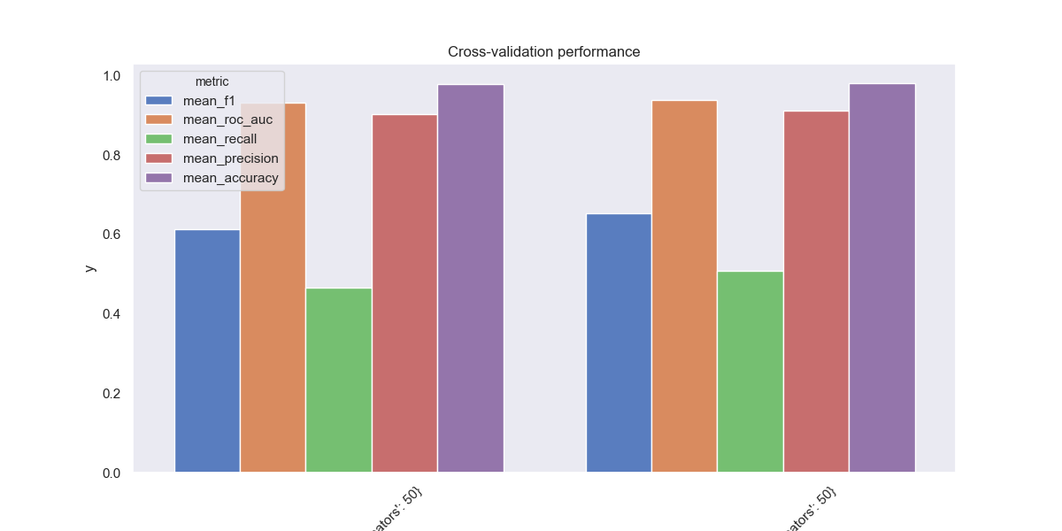
This model exchanges recall in order to become much more precise. Instead of labeling everything as fraud, this model misses about 50% of all fraud cases. But when it does label a transaction as fraudulent, there’s a high likelihood (90%+) that it’s actually fraud.

A note about class imbalance

Only 3.5% of the samples in training_transactions.csv were fraudlent credit card transactions, meaning that any model that always predicted “no fraud” 100% we would exptect to be about 96.5% accurate. This is unacceptable, so we assign class weights to the fraud/no fraud samples in the training set to increase the penalty of a classifier for predicting false negatives.

Sklearn provides a very simple entrypoint for modifying class weights on most of its estimators. I recommend using the setting 'balanced' lest you want the individual class weights to become yet another hyperparameter:

model = ExtraTreesClassifier(class_weight='balanced')

There are many good Google-able resources for how to train models in the face of severe class imbalance. I always recommend studying a confusion matrix and calculating precision (the rate at which predicted fraud cases are actually fraudulent) and recall (the number of fraudulent cases identified). False positives and false negatives have a variable cost depending on your industry, and the job of the data scientist is often to minimize the total cost incurred by both.

Lessons learned

At the end of the day, I was able to develop a data pipeline that gave me both decent model performance and the ability to get model predictions from a one-liner:

preds = model.predict(pipeline.transform(read_csv('test_transactions.csv')))

1. Sklearn does not provide a good API for changing data types, and building a custom Transformer to cast all categorical features astype(str) does not play nicely with downstream Transformers, hence my decision to preprocess string- and numerically-valued categorical features separately. Sklearn transformers generally transform input data X into numpy arrays, even when X is a pandas.DataFrame.
2. While you can use two ColumnTransfomers in succession, I would not recommend it. The default behavior of a ColumnTransfomer is to apply a Pipeline Transformer to a subset of columns in X and return only that transformed feature subset. I’m referring to the parameter remainder, whose default is the string 'drop'. You can specify remainder = 'passthrough' and have the transformer return all features, both transformed and untransformed. But a more easily-understood way to write feature-specific transforms is to define separate ColumnTransformers for each group of features that requires a separate processing pipeline and then using FeatureUnion to horizontally concatenate them. This approach has the added benefit of selecting, in the end, only the subset of features you intend to use for modeling purposes and excludes any features that were not explicitly passed into the pipeline.
3. Related to 2., it is better to explicitly define which features from your data, X, will be used for modeling than implicitly state which features will not be used for modeling. For example, the training data contains a date field, TransactionDT. Chaining multiple ColumnTransformer each with remainder=True runs the risk of including TransactionDT unless we specifically exclude that feature. The transaction date in the training set will be prior to a future test set (unless we extract date-agnostic features like time of day or day of week), so it makes no sense to keep TransactionDT for predictive purposes. Instead, define the features you want to use.

Manual feature selection and engineering can become both time intensive, arbitrary, and based on naive univariate tests between a target variable Y and individual covariates X_i. Two automatic feature selection methods (e.g. those in the sklearn.feature_selection module) will most often result in different sets of feature sets.