Joining Type II change tables and logistics industry data
Logistics industry 101
Working as a consultant at Aptitive, my longest-standing client was a large North American logistics company. The logistics industry is huge in Chicago, an industry that dates back to a time when Chicago served as major crossroads and trading hub connecting the East Coast to the West, the Great Lakes to the Mississippi River. Logistics is a huge industry nationwide - trucking is the most common profession in 29 states in the US according to the Bureau of Labor Statistics - and there is virtually no centralization among trucking companies. There isn’t a meaningful Amazon or Apple of hauling freight. This makes the industry simultaneously amenable to technological advancement, but also full of complicated, decentralized data.
Here’s what I learned working with my client: the logistics industry is in the midst of a massive transformation, from a federation of human actors making gut-instinct choices into an automated system driven by subject matter experts who know a thing or two about the complexities of transportation management service data structures.
Before we get into code, we’ll need some useful industry terms:
- A logistics company’s customers are their clients who use the logistics firm to move their freight. Confusingly, customers are also referred to in the industry as shippers.
- Carriers are the people moving freight, e.g. truckers or UPS.
- Freight brokering: In Chicago, there are many logistics brokerage firms who basically serve as a spot market for shipping rates. A customer tells the brokerage about their freight, and a broker then quotes the customer a rate. The brokerage makes a profit by finding a carrier who submits a bid to move the freight for less money than what the brokerage charged the customer to move the freight. Brokering involves reserving an entire truck for the customer’s freight.
- Less-than-truckload shipping (LTL): if brokers reserve entire trucks, then LTL shipping is when customer’s freight only takes up a portion of a truck, so that multiple customers’ freight can move on the same truck at once. Think of Uber Black vs Uber Pool. LTL usually comes with lower profit margins for a logistics company than brokered loads, but LTL is easier to plan for because customers typically book LTL freight far in advance, on a recurring basis.
- Loads are units of customer freight.
- Different transportation modes for moving loads, like rail, ocean barge, airplane, are configured on a load-by-load basis. The majority of the time we’re
talking about freight moved by trucks. Trucks-based modes are dry van (i.e. a regular, unrefrigerated truck), reefer (a refrigerated truck),
intermodal (trailers that can travel by rail and truck), etc.
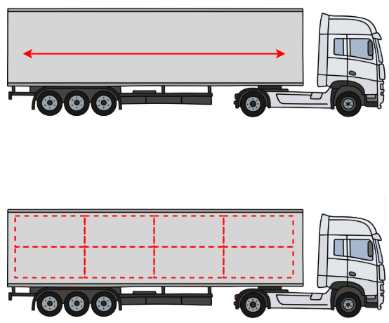 Full truckload freight (top) vs LTL freight (bottom)
- Lanes are (origin, destination) pairs that describe where a load is moving. It’s possible to for one load to move across multiple lanes, for example, if
a customer needs freight to be picked up from two separate warehouses and dropped off at a single destination.
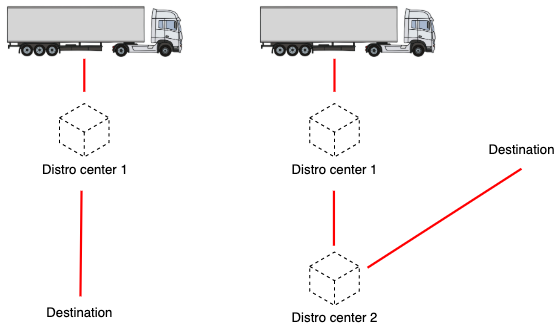 A load on a single lane (left) vs a multi-lane load (right)
So, in a sentence:
"Freight brokerages or LTL shippers assign loads a particular mode and then find carriers who can move those loads across lanes."
Type I vs Type II changes: reflecting changes in a database
Getting back to data - not all data warehouses are created equally, especially when it comes to their ability to track the history of particular entities over time. Here, by entity I’m referring to any object of business value (a load, a lane, a mode, a carrier, etc.). Now, the history of a load can be quite complicated. A load can be reconfigured by any number of logistics representatives; a load’s transportation mode or total weight might need to be updated if a customer decides to change the contents of the load. The destination may need to change if supply or demand for the customer’s products change in a particular region overnight.
Suppose we’re working for our logistics client, and they have just one table called Loads
containing all of the details for the client’s loads. When a logistics representative needs to change, say, a load’s transportation mode, there are a few different ways to reflect their changes in the Loads table.
Type I changes
Tables that using Type I changes is the easiest, but also the most naive, way to store changes in a database. Type I changes
are just updates to existing records so that tables retain their one row = one entity rule. If the Loads
table uses Type I changes, then one row = one load. Type I tables usually have an updated_by_user and an updated_date that represent
which database user updated some aspect of the load, and when.
Example: suppose a load_id 123 was created with a weight of 30,000 lbs, but the customer
decided they needed an extra 5,000 lbs shipped a couple of days later:
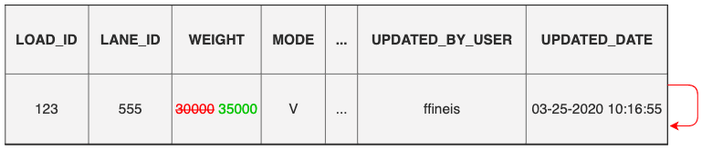 Updating a load's weight in place with a Type I change.
So Type I changes are updates in place. The main benefit of Type I changes are that they maintain the 1-1 mapping of rows to loads. The drawback is that you lose the ability to track history. All you know is which user made the recent change, and when that change happened. We don’t necessary know what changes occurred.
You could “beef up” your Type I changes to apply the updated_by_user and updated_date concept to every field, so, adding
weight_updated_by_user and weight_updated_date fields like this:
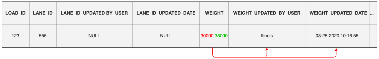
But this is pretty awkward. And moreover, at any given time we’re only retaining the most recent change in each field, so this solution is still only a half-measure towards being able to track the full changelog history of a load.
Type II changes
Instead of updating individual records, what if we just inserted a new version of each record as those changes arrived? The Type II change
for our load that started at 30,000 lbs and increased to 35,000 lbs would would appear
as a near-duplicate record, but with the updated weight and a effective_date field telling us when the change was in effect.
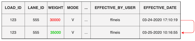 Updating a load's weight with a Type II insert.
Leveraging Type II changes, the meaning of each record in a table has changed. No longer is one record = one entity. One record is
one version of one entity. Now load_id 123 can show up multiple times. The grain of the table has changed.
We can even figure out the exact time window that each version of each record was good for by using SQL’s lead function
to tie the next version’s effective_date at time t + 1 to the version at time t. That is, a particular
version of an entity is only in effect until the next version of that same entity comes in at a later time. In order
to give each version of each load a [start, end) window, we would do the following:
select *
    , effective_date as start_date
    , lead(effective_date, 1) over (partition by load_id order by effective_date) as end_date
from Loads
order by start_date asc;| load_id | lane_id | weight | mode | start_date | end_date |
|---|---|---|---|---|---|
| 123 | 555 | 30000 | V | 03-24-2020 17:10:19 | 03-25-2020 10:16:55 |
| 123 | 555 | 35000 | V | 03-25-2020 10:16:55 | NULL |
In this way, we keep track of when exactly each version of a load was in effect. A record whose end_date is NULL indicates that this record is the currently active record, because
it has yet to be superseded by a more recent version.
While Type II changes add costs (e.g. need for a bigger server, cloud host wants more money more for storage), this strategy gives our client the ability to recreate each unique version of each load at any given point in time. We have traded power for complexity, namely, in that we have made our table more granular.
Joining in time with Type II changes
We’d like to set our client up with Type II enabled tables. But a problem has arisen. If we were previously joining two tables on a simple (primary key, foreign key) match, and if Type II changes duplicate each primary/foreign key for every distinct version of each record, then joining on keys will join every change in table 1 to every change in table 2! In data modeling, this is called a cartesian (or cross) join, and it’s a bad thing if it’s not intentional.
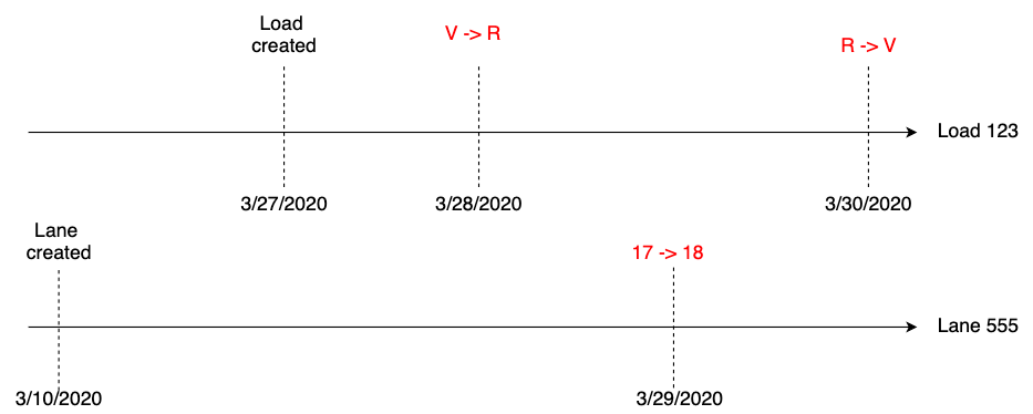
Suppose we have some sample data that includes a load (load_id 123). This load is assigned to lane_id 555. This load has three different versions:
load_id 123gets created on 3/27/2020 with the ‘V’ (short for “dry van”) transportation mode.- This load’s mode gets changed on 3/28/2020 to ‘R’ (short for “refrigerated”).
- Two days later (on 3/30/2020), a logistics representative realizes that the load is not actually a reefer load after all, but still actually a dry van load.
Also suppose that there are two versions of lane_id 555:
- This lane was supposed to represent the lane between Tulsa, Oklahoma (
city_id 10) and Portland, Maine (city_id 18). But when the lane was created on 3/10/2020, it is assigneddestination_city_id = 17. - On 3/29/2020 a user realizes the mistake:
city_id 17is Portland, Oregon, not Portland, Maine. Hey, honest mistake. They create a new version oflane_id 555with the correct destination.
Now a logistics analyst wants to join the Loads and Lanes tables (suppose tgat lane_id is a foreign key contained in the Loads table). They notice the cartesian:
select l.load_id
    , l.lane_id
    , l.mode
    , ln.origin_city_id
    , ln.destination_city_id
    , l.effective_date as load_effective_date
    , ln.effective_date as lane_effective_date
from Loads l
inner join Lanes as ln
    on l.lane_id = ln.lane_id
order by load_effective_date asc;| load_id | lane_id | mode | origin_city_id | destination_city_id | load_effective_date | lane_effective_date |
|---|---|---|---|---|---|---|
| 123 | 555 | V | 10 | 17 | 03-27-2020 00:00:00 | 03-10-2020 00:00:00 |
| 123 | 555 | V | 10 | 18 | 03-27-2020 00:00:00 | 03-29-2020 00:00:00 |
| 123 | 555 | R | 10 | 17 | 03-28-2020 00:00:00 | 03-10-2020 00:00:00 |
| 123 | 555 | R | 10 | 18 | 03-28-2020 00:00:00 | 03-29-2020 00:00:00 |
| 123 | 555 | V | 10 | 17 | 03-30-2020 00:00:00 | 03-10-2020 00:00:00 |
| 123 | 555 | V | 10 | 18 | 03-30-2020 00:00:00 | 03-29-2020 00:00:00 |
All of the changes in Loads are being applied to all of the changes in Lanes! Since the first version of load_id 123
is only effective between 3/27/2020 and 3/28/2020 and the updated version of lane_id 555 is effective only starting
on 3/29/2020, so the original version of this load could not possibly have been tied to the updated version of the lane.
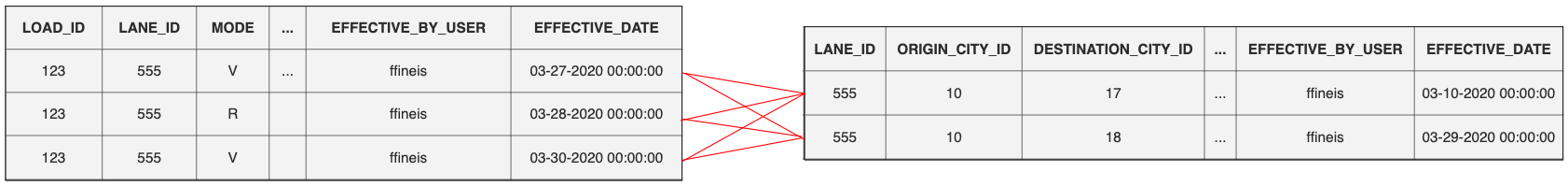 Joining Type II data without using effective windows leads to undesirable cartesians.
Joining using effective windows
Clearly, we need to be able to join not only on primary/foreign keys but to be able to join across time. To do this,
each load_id and each lane_id need an effective window explaining the time period each record is good for. There should really only be four records:
 The complete history of load_id 123 while joined to lane_id 555.
- (1 record) The original version of
load_id 123joins to the original version oflane_id 555 - (2 records) The second version of
load_id 123(withmode = 'R') should be joined to both versions oflane_id 555(withdestination_city_id = 17and18) - (1 record) The final version of
load_id 123(returning tomode = 'V') should be joined to the final version oflane_id 555.
The easiest way tack on effective windows to each table is to use common table expressions (CTEs). CTEs
allow you to write and name select statements and use them as if they were database tables. Most SQL dialects support CTEs in some form. Now,
we’ll continue to join Loads to Lanes using Loads.lane_id = Lanes.lane_id, but now we filter down to load_id records whose effective windows overlap
with corresponding lane_id effective windows.
with cte_loads as (
    select *
    , effective_date as load_start_date
    -- cast NULL effective_dates (indicating current record) to far in the future.
    , nvl(lead(effective_date, 1), '2099-01-01'::date) over (partition by load_id order by effective_date) as load_end_date
    from Loads)

, cte_lanes as (
    select *
    , effective_date as lane_start_date
    , nvl(lead(effective_date, 1), '2099-01-01'::date) over (partition by lane_id order by effective_date) as lane_end_date
    from Lanes)

select l.load_id
    , l.lane_id
    , l.mode
    , ln.origin_city_id
    , ln.destination_city_id
    , l.load_start_date
    , l.load_end_date
    , ln.lane_start_date
    , ln.lane_end_date
from cte_loads l
inner join cte_lanes as ln
    -- join on primary/foreign key match
    on l.lane_id = ln.lane_id
    -- join on effective window overlap
    and ((load_start_date >= lane_start_date and load_start_date < lane_end_date)
        or (load_end_date >= lane_start_date and load_end_date < lane_end_date)
        or (lane_start_date >= load_start_date and lane_start_date < load_end_date)
        or (lane_end_date >= load_start_date and lane_end_date < load_end_date))
order by load_start_date asc;| load_id | lane_id | mode | origin_city_id | destination_city_id | load_start_date | load_end_date | lane_start_date | lane_end_date |
|---|---|---|---|---|---|---|---|---|
| 123 | 555 | V | 10 | 17 | 03-27-2020 00:00:00 | 03-28-2020 00:00:00 | 03-10-2020 00:00:00 | 03-29-2020 00:00:00 |
| 123 | 555 | R | 10 | 17 | 03-28-2020 00:00:00 | 03-30-2020 00:00:00 | 03-10-2020 00:00:00 | 03-29-2020 00:00:00 |
| 123 | 555 | R | 10 | 18 | 03-28-2020 00:00:00 | 03-30-2020 00:00:00 | 03-29-2020 00:00:00 | 01-01-2099 00:00:00 |
| 123 | 555 | V | 10 | 18 | 03-30-2020 00:00:00 | 01-01-2099 00:00:00 | 03-29-2020 00:00:00 | 01-01-2099 00:00:00 |
Now we only join together versions of loads to versions lanes that would have been possible to occur over time.
What is going on in this join condition? Well, there are only four possible ways that two 2-sided windows can intersect,
so that’s what each of the lines in the and join condition above are addressing:
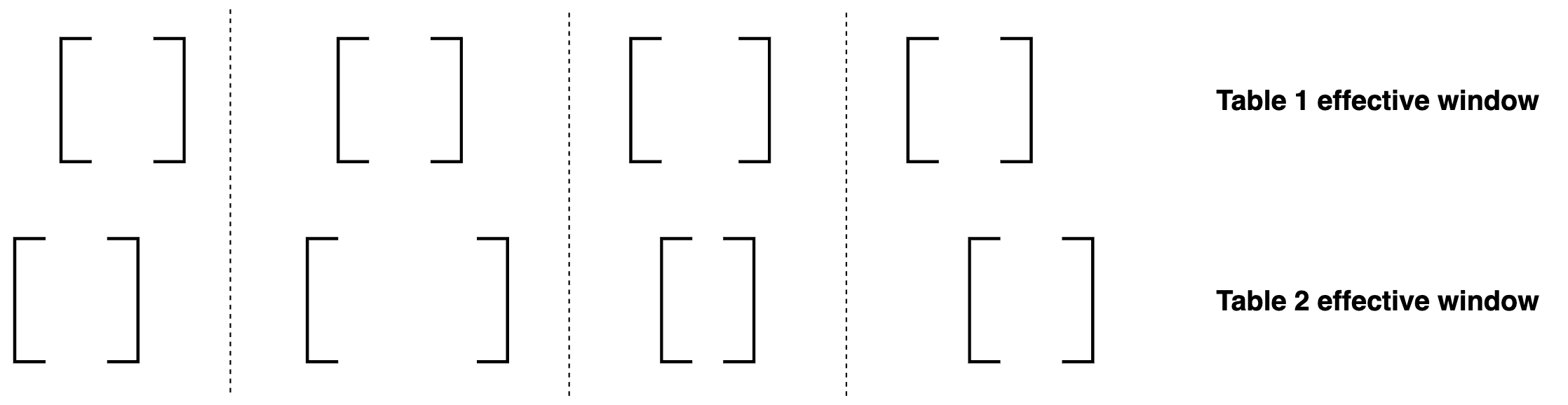 The four possible ways for two effective windows to overlap.
Awesome, now our client’s analysts can track the full history of all loads and lanes, and now they can even
do things like track how many mistakes were made on each load, or how long it took for a load to change from
between any two statuses; Type II data is much richer than a naive updated_date timestamp.
Selecting only currently-valid records from Type II table joins
The effective window join pattern presented above is great for querying the entire temporal history of changelog data across separate tables, but what if we just want a current snapshot of the joined Type II tables? That is, we only want joined changelog records that apply at the current moment in time, not those from the past.
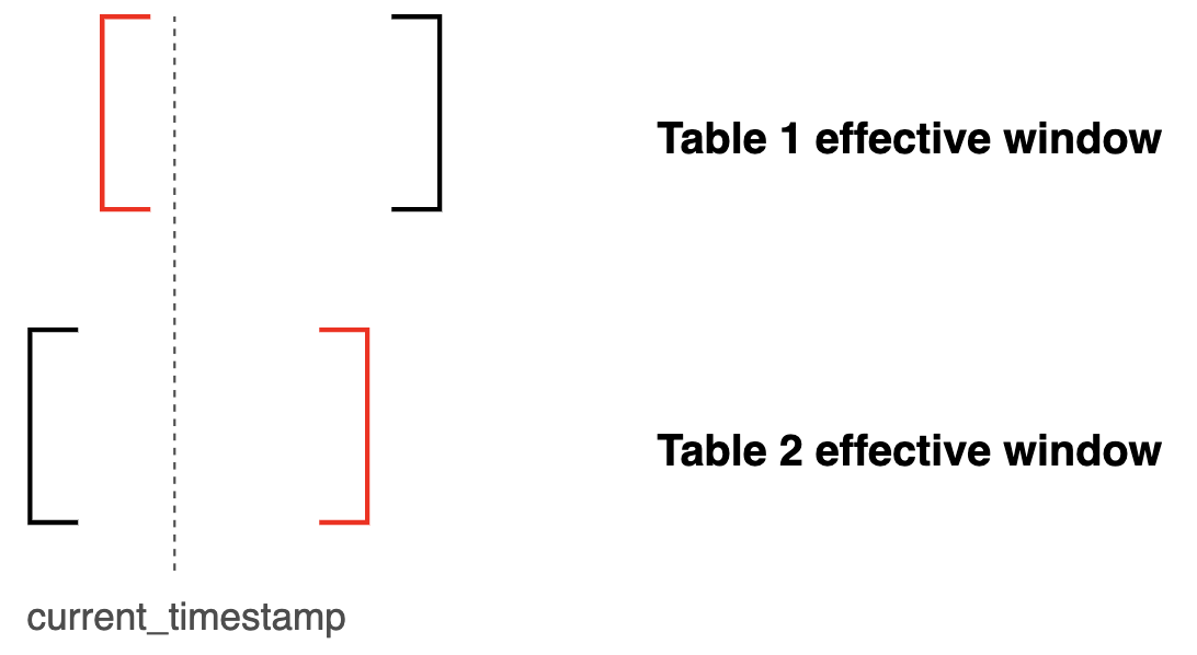
Logically, two joined Type II records are only valid at the current moment in time if the latest start_date
of either constituent record is before the current_timestamp while simultaneously the earliest end_date of either constituent
record is after the current point in time.
with cte_loads as (...)

, cte_lanes as (...)

select l.load_id
    , l.lane_id
    , l.mode
    , ln.origin_city_id
    , ln.destination_city_id
    , l.load_start_date
    , l.load_end_date
    , ln.lane_start_date
    , ln.lane_end_date
from cte_loads l
inner join cte_lanes as ln
    on l.lane_id = ln.lane_id
    and greatest(load_start_date, lane_start_date) <= current_timestamp
    and least(load_end_date, lane_end_date) >= current_timestamp
order by load_start_date asc;
Now this query limits our results to only the version of loads that join to lanes (in time) whose joint effective windows include the current time. What I’m describing looks like this:
Now our client’s logistics analysts can freely select either a completely versioned history of all loads and lanes, or, only what the state of loads and lanes look like at the current point in time.
End
Thanks for reading! Don’t hesitate to get in touch if your organization is having trouble implementing, scaling, or migrating to fully-versioned data.